Simplifying payments with linear programming
Update: I have built a demo webapp implementing the solution presented here. You should try it!
Imagine you have a group of $n$ friends and that you regularly go out for drinks with them (say, a couple of times a week). At each of these meetings, a different member of the group pays for the bill, but you keep track of who consumed what (by using one of these popular apps, for example). You can expect that, after a month or so, everyone is going to owe everyone some amount of money. Settling these debts will involve a cumbersome sequence of up to $n(n-1)$ payments from each member to another. The question which obviously arises is then:
Can we reduce the number of transactions to a minimum while ensuring that everyone gets paid what he or she is owed?
The answer yes, but finding the optimal solution can take you a lot of time. As has been noted elsewhere, this seemingly inoffensive problem is actually NP-hard. Many people have proposed many different heuristics to approach this problem (see this Stackoverflow question). My problem with these solutions is simply that they are not as elegant as I would like them to be.
Linear programming
In this post, I am going to show you a completely different approach to solve this problem by using Linear Programming. A standard formulation of an LP is: $$ \begin{aligned} & \min_{x \in \mathbb{R}^N} & & c^Tx \\ & \text{s.t} & & Ax \leq b \\ &&& x \geq 0 \end{aligned} $$
where $c \in \mathbb{R}^N$, $A$ is matrix of size $m \times N$ and $b \in \mathbb{R}^m$ ($\geq$ and $\leq$ work as element-wise inequalities). LP is a mature technology, with many solvers available under both commercial and open source licenses, that can solve problems involving thousands of variables using a desktop computer in under a minute (Boyd and Vandenberghe 2004). In what follows, I will show you how to leverage this technology to solve the problem we are tackling.
Mathematical formulation of the problem
We will describe the debts within the group by a matrix $D$ such that $d_{ij} \geq 0$ is the amount of money that the $i$-th member owes to the $j$-th member: $$ D = \begin{pmatrix} 0 & d_{12} & \dots & d_{1N} \\ d_{21} & 0 & \dots & d_{2N} \\ \vdots & \vdots & \ddots & \vdots \\ d_{N1} & \dots & d_{NN-1}& 0 \end{pmatrix} $$
The diagonal is full of 0’s because nobody owes himself, but other than that, we are assuming that this matrix is very dense, so that $d_{ij} > 0$ for most of the $i \neq j$ pairs.
Under this description, our aim is then to find a different matrix $X$ that has the least possible number of entries $x_{ij} > 0$, but that satisfies the constraint imposed by the problem. The constraints can be cast as $$ \forall i: \underbrace{\sum_j x_{ji}}_{\text{owed to }i\text{ under }X} - \underbrace{\sum_j x_{ij}}_{\text{owed by }i\text{ under }X} = \underbrace{\sum_j d_{ji}}_{\text{owed to }i\text{ under }D} - \underbrace{\sum_j d_{ij}}_{\text{owed by }i\text{ under }D} $$
We can express this succinctly using linear algebra: $$ (X^T - X)1_n = (D^T - D)1_n $$
Note that the function $f_c(X) = (X^T - X)c$ is linear in $X$, $\forall c \in \mathbb{R}^n$, since $\forall \alpha, \beta \in \mathbb{R}$: $$ \begin{aligned} f_c(\alpha X + \beta Y) &= [(\alpha X + \beta Y)^T - (\alpha X + \beta Y)]c \\ &= \alpha(X^T - X)c + \beta(Y^T - Y)c \\ &= \alpha f_c(X) + \beta f_c(Y) \end{aligned} $$
Using the above definitions, we can now formally state our optimization problem $$ \begin{aligned} & \min_{X \in \mathbb{R}^{n\times n}} & & \|X\|_0 \\ & \text{s.t} & & (X^T - X)1_n = b \\ &&& x_{ii} = 0, \forall i \\ &&& x_{ij} \geq 0, \forall i \neq j \end{aligned} $$
where we have defined $r \triangleq (D^T - D)1_n$, to highlight the fact that this is the only way our problem depends on $D$. In other words, we could do the same analysis if someone gave us $b$ instead of $D$. Also, $\|X\|_0$ is the number of non-zero components in $X$.
Now, if we wanted to say that this looks like an LP, we would run into two issues:
$X$is a matrix, not a vector$\|\cdot\|_0$is not a linear function (nor differentiable, nor continuous)
The first issue is actually easier to deal with, so we’ll start with that one.
Thinking in terms of vectors instead of matrices
As you may know from linear algebra courses, the space of matrices with real entries of size $r\times c$, $\mathbb{R}^{r\times c}$, is isomorphic to $\mathbb{R}^{rc}$. One isomorphism is the function: $$ vec: \mathbb{R}^{r\times c} \to \mathbb{R}^{rc} $$
such that $\forall M \in \mathbb{R}^{r\times c}$, $v = vec(M)$ is a vector of size $rc$ formed by stacking the columns of $M$.
Given the above, we could therefore work with $x = vec(X)$. Since this is an isomorphism, and the restriction is linear in $X$, we know that: $$ \exists A \in \mathbb{R}^{n\times n^2}, \forall X \in \mathbb{R}^{n\times n}: Avec(X) = (X^T - X)1_n $$
This is all good, but we could further exploit the structure of the problem in order to make this translation into vectors more efficient. Indeed, recall that we are looking for a matrix with a diagonal of zeroes. Therefore, instead of working with vectors in $\mathbb{R}^{n^2}$ and setting up restrictions for enforcing a zero diagonal, we could just remove the diagonal from our vector representation. This way, we reduce the number of degrees of freedom and the number of restrictions.
Thus, let us define the function $$ vec^*: \mathbb{R}^{n\times n} \to \mathbb{R}^{n(n-1)} $$
such that $v = vec^*(M)$ is a vector of size $n(n-1)$ where the columns of $M$ are stacked on top of one another, but the elements of the diagonal are removed. If we restrict the domain of $vec^*$ to the set $$ \mathcal{D}_0 = \{M \in \mathbb{R}^{n\times n}: \text{diag}(M) = 0_n\} $$
then $$ vec^*: \mathcal{D}_0 \to \mathbb{R}^{n(n-1)} $$
is an isomorphism. Hence, $$ \exists A \in \mathbb{R}^{n\times n(n-1)}, \forall X \in \mathcal{D}_0: Avec^*(X) = (X^T - X)1_n $$
Indeed, the matrix $A$ can be constructed for any $n \geq 2$. I have built an R package that implements the approach I describe in this blog called minTX and which is available from Github. It uses the lpSolve package, which is an interface to the lp_solve solver. minTX also has all the helper functions needed for the matrix <-> vector conversions and for building the constraint matrix. So, let me show you how $A$ looks like for $n=3$:
library(minTX)

n = 3
A = get_const_matrix(n)
A
##      [,1] [,2] [,3] [,4] [,5] [,6]
## [1,]    1    1   -1    0   -1    0
## [2,]   -1    0    1    1    0   -1
## [3,]    0   -1    0   -1    1    1
Let’s check that this weird construction works as it should
# get a random matrix with positive coefficients and diag = 0
M = matrix(rexp(n*n, 0.1), nrow = n); diag(M) = rep(0, n)
all.equal(colSums(M) - rowSums(M), as.vector(A %*% mat_2_vec(M)))
## [1] TRUE
And the same, but for $n = 20$:
n = 20
M = matrix(rexp(n*n, 0.1), nrow = n); diag(M) = rep(0, n)
all.equal(colSums(M) - rowSums(M), as.vector(get_const_matrix(n) %*% mat_2_vec(M)))
## [1] TRUE
From a nonlinear target to a linear one
Okay, so we’ve managed to go from matrices to vectors, so that our optimization problem now looks like: $$ \begin{aligned} & \min_{x \in \mathbb{R}^{n(n-1)}} & & \|x\|_0 \\ & \text{s.t} & & Ax = b \\ &&& x \geq 0 \end{aligned} $$
The fact that the constraint is expressed as an equality is of no concern, because one can always express an equality as a pair of inequalities.
Now, in order to deal with the fact that the target is nonlinear, we will introduce the following change in the objective function: $$ \begin{aligned} & \min_{x \in \mathbb{R}^{n(n-1)}} & & \|x\|_1 \\ & \text{s.t} & & Ax = b \\ &&& x \geq 0 \end{aligned} $$
where $\|\cdot\|_1$ is the $L^1$-norm. Since we require that $x \geq 0$, we can again rewrite this as $$ \begin{aligned} & \min_{x \in \mathbb{R}^{n(n-1)}} & & c^T x \\ & \text{s.t} & & Ax = b \\ &&& x \geq 0 \end{aligned} $$
with $c = 1_{n(n-1)}$. This is now a linear program.
It also a fundamentally different problem: we are now minimizing the total amount of transactions, which is of course not the same as minimizing the total number of transactions.
However, the work by Donoho and Tanner (2005) gives an answer: if there exists a sufficiently sparse representation for $x$, then the solution to both problems is the same. This is one of many results of the much interesting field of Compressed Sensing, of which I know very little of, so I am not even going to try to give an introduction. However, if you are familiar with the Lasso technique in statistics, you might get a sense of what is going on under the hood here.
Experiments!
Circular debts
In this case, we assume that the matrix $D$ is such that we can find a circular arrangement of the participants in which every person pays an amount $s$ to the person in front, and therefore receives the same amount from the person behind. We know in advance that the optimal solution to this system is that no transaction needs to be made.
suppressPackageStartupMessages(library(igraph))
suppressPackageStartupMessages(library(ggraph))

# function to obtain circular payment matrix
get_cir_D = function(n, s){
  D = rbind(cbind(rep(0, n-1), s*diag(n-1)), rep(0,n))
  D[n,1] = s
  return(D)
}

# make and plot matrix of size 8
n = 8; s = 10
D = get_cir_D(n, s)

graph_from_adjacency_matrix(D, mode = "directed", weighted = TRUE) %>%
  ggraph(layout = "circle") +
  geom_edge_link(aes(label = weight), angle_calc = 'along', label_dodge = unit(2.5, 'mm'), arrow = arrow(length = unit(4, 'mm'))) +
  geom_node_point(size = 5) +
  theme_graph()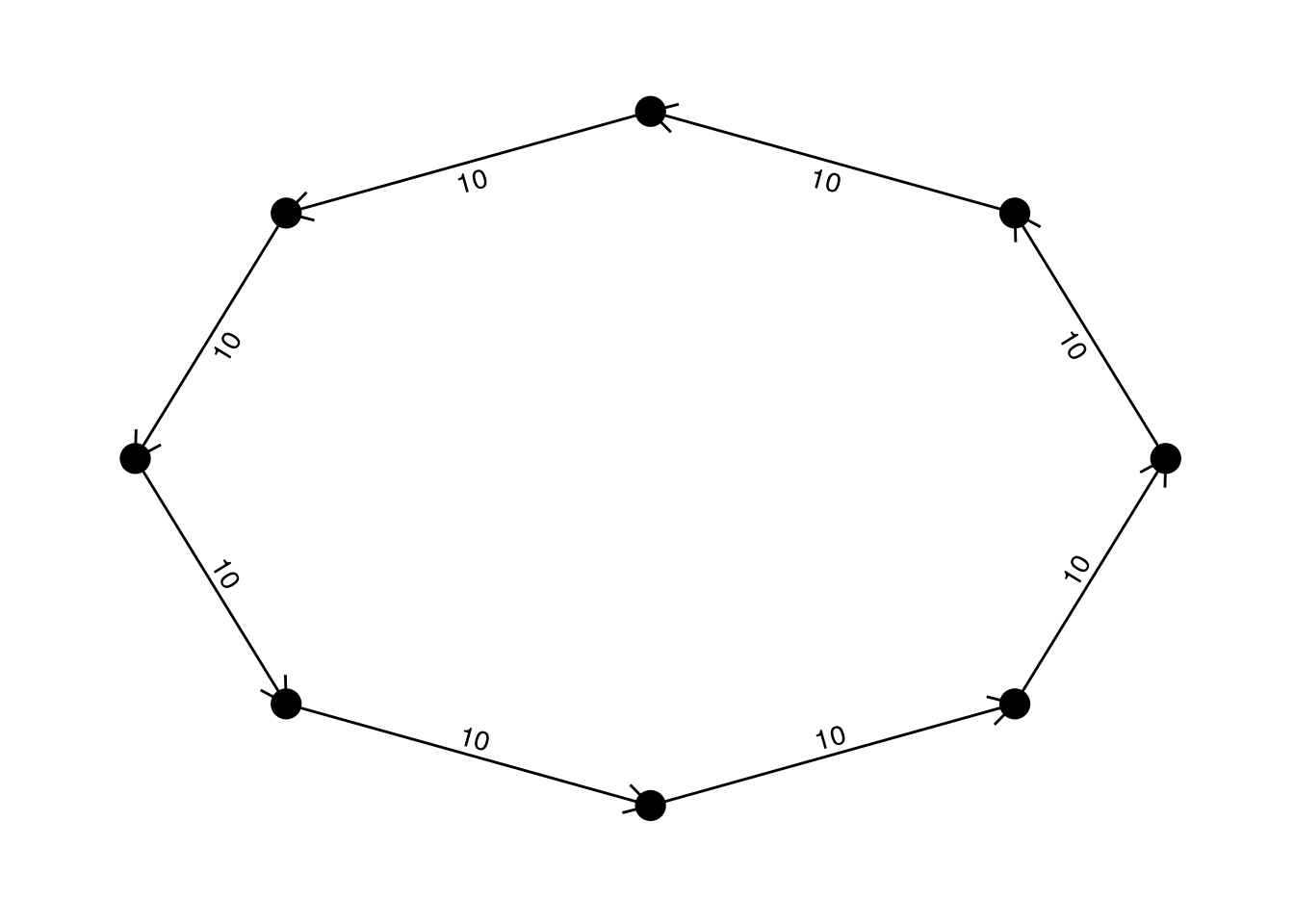
Let’s see if our procedure finds the optimal allocation
solve_min_TX(D)
## Success: the objective function is 0
##      [,1] [,2] [,3] [,4] [,5] [,6] [,7] [,8]
## [1,]    0    0    0    0    0    0    0    0
## [2,]    0    0    0    0    0    0    0    0
## [3,]    0    0    0    0    0    0    0    0
## [4,]    0    0    0    0    0    0    0    0
## [5,]    0    0    0    0    0    0    0    0
## [6,]    0    0    0    0    0    0    0    0
## [7,]    0    0    0    0    0    0    0    0
## [8,]    0    0    0    0    0    0    0    0
Great! The solution found by minTX is indeed the optimal one.
Dense payment matrix
Now, let us try with a dense matrix:
set.seed(1313)

# function to obtain a random dense payment matrix
get_dense_D = function(n, s){
  D = matrix(rexp(n*n, 1/s), nrow = n)
  diag(D) = rep(0, n)
  return(D)
}

# make and plot matrix of size 8
D = get_dense_D(n, s)

graph_from_adjacency_matrix(D, mode = "directed", weighted = TRUE) %>%
  ggraph(layout = "circle") +
  geom_edge_link(aes(label = format.default(weight, digits = 1)), angle_calc = 'along', label_dodge = unit(2.5, 'mm'), arrow = arrow(length = unit(4, 'mm'))) +
  geom_node_point(size = 5) +
  theme_graph()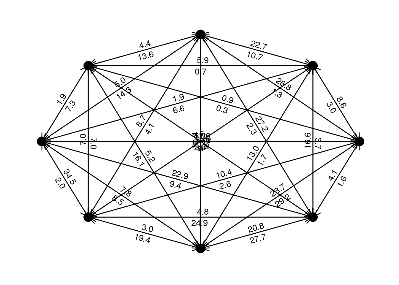
It’s a mess, of course! Again, lets solve this using our procedure, making sure that it returns a valid payments matrix:
X = solve_min_TX(D)
## Success: the objective function is 151.0473
all.equal(colSums(D) - rowSums(D), colSums(X) - rowSums(X))
## [1] TRUE
Okay, now let’s take a look at the graph implied by the matrix produced by minTX:
graph_from_adjacency_matrix(X, mode = "directed", weighted = TRUE) %>%
  ggraph(layout = "circle") +
  geom_edge_link(aes(label = format.default(weight, digits = 1)), angle_calc = 'along', label_dodge = unit(2.5, 'mm'), arrow = arrow(length = unit(4, 'mm'))) +
  geom_node_point(size = 5) +
  theme_graph()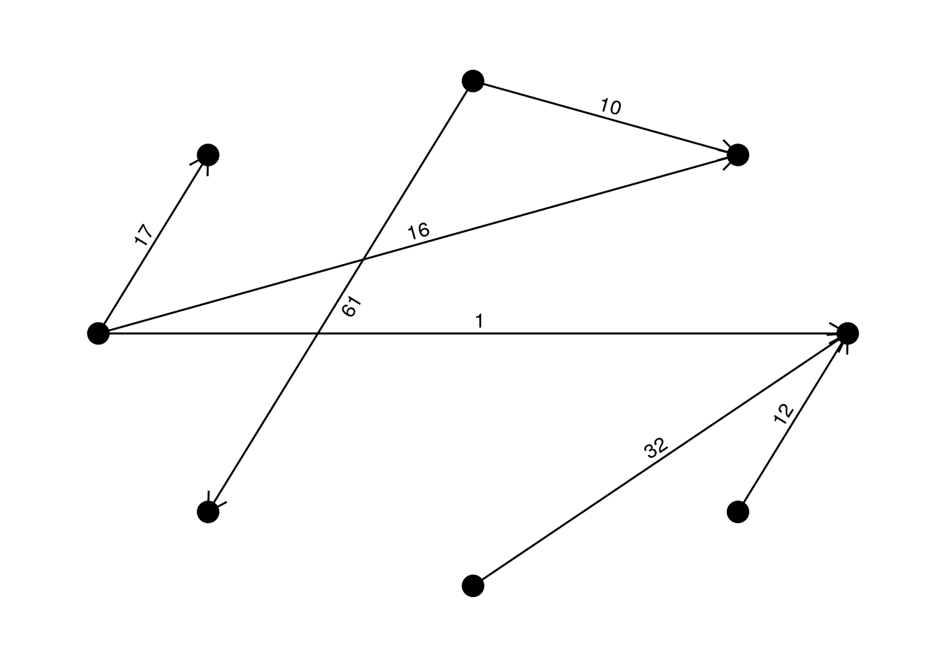
Much simpler than before, isn’t it? In fact, we went down from 56 to barely 7 payments!
Let’s try the same dense matrix setup, but now with many more participants, and see how long it takes for our procedure to find a solution
n = 100

# make matrix
D = get_dense_D(n, s)

# solve
start.time = Sys.time()
X = solve_min_TX(D)
## Success: the objective function is 6407.031
print(Sys.time() - start.time)
## Time difference of 0.5953553 secs
Now, we went down from 9900 to 99 payments. And just to make sure, lets check the consistency:
all.equal(colSums(D) - rowSums(D), colSums(X) - rowSums(X))
## [1] TRUE
Conclusions and future work
In this post I have demonstrated a different approach to the problem of minimizing the number of payments between a set of counterparties, by leveraging the power of widely available LP solvers. I believe that this approach is valuable because it has the potential to scale to thousands of participants if we exploited the sparsity of the constraint matrix.
In the future, I would like to give more formal guarantees on the ability of the procedure to recover the sparsest solution. I would also like to improve the computational implementation, which is still very naive.
If you are interested in discussing about this, feel free to leave a comment and/or to contact me.
References
Boyd, Stephen, and Lieven Vandenberghe. 2004. Convex Optimization. Cambridge university press.
Donoho, David L, and Jared Tanner. 2005. “Sparse Nonnegative Solution of Underdetermined Linear Equations by Linear Programming.” Proceedings of the National Academy of Sciences of the United States of America 102 (27). National Acad Sciences: 9446–51.