Visualizing Fourier series in 2D and 3D

March 9, 2018

In this post, I will give a brief description of real valued Fourier series in higher dimensions, with some neat plots. I started reading about Fourier series because in the 1D case they are useful for extracting periodic patterns from time series data. However, I ended up fascinated by the pretty pictures one could get by plotting random 2D series, or by the periodic videos made by “walking” along a 3D space “painted”" with a Fourier series.

Fourier series in higher dimensions

In this section I will be loosely following chapter 8 of the lecture notes prepared by Prof. Brad Osgood for his course The fourier Transform and its Applications, which can be found here.

A function $f:\mathbb{R}^d \to \mathbb{C}$ is said to be periodic with period 1 if $\forall \boldsymbol{x} \in \mathbb{R}^d, \mathbb{Z}^d$ : $$ f(\boldsymbol{x} + \boldsymbol{n}) = f(\boldsymbol{x}) $$

The set $\mathbb{Z}^d$ is known as the $d$ -dimensional integer lattice, whose elements are $d$ -tuples of integers: $$ \mathbb{Z}^d = \{\boldsymbol{n} = (n_1, ..., n_d): n_1, ..., n_d \in \mathbb{Z}\} $$

Now, suppose that $f$ is a periodic function of period 1 which is also square-integrable; i.e., $f \in L^2([-1, 1]^d)$ . This means that: $$ \int_{[-1, 1]^d} |f(\boldsymbol{x})|^2 d\boldsymbol{x} < \infty $$

In this case, we know there exists a Fourier series: $$ s(\boldsymbol{x}) = \sum_{\boldsymbol{n}} c_{\boldsymbol{n}}e^{2\pi i \boldsymbol{n} \cdot \boldsymbol{x}} $$

where $c_{\boldsymbol{n}} \in \mathbb{C}^d$ , such that: $$ \int_{[-1, 1]^d} |f(\boldsymbol{x}) - s(\boldsymbol{x})|^2 d\boldsymbol{x} = 0 $$

This is a direct consequence of the fact that the set $\{e^{2\pi i \boldsymbol{n} \cdot \boldsymbol{x}}: \boldsymbol{n} \in \mathbb{Z}^d \}$ is a basis for the space $L^2([-1, 1]^d)$ .

Fourier series of real-valued functions

In the special case where $f$ is real-valued, when can greatly reduce the amount of coefficients needed to represent $f$ . Indeed, if the function is real-valued, then $\forall \boldsymbol{x} \in \mathbb{R}^d$ : $$ \begin{aligned} 0 &= \Im(f(\boldsymbol{x})) \\ &= \Im(s(\boldsymbol{x})) \\ &= \Im\left( \sum_{\boldsymbol{n}} c_{\boldsymbol{n}}e^{2\pi i \boldsymbol{n} \cdot \boldsymbol{x}} \right) \\ &= \sum_{\boldsymbol{n}} \Im( c_{\boldsymbol{n}}e^{2\pi i \boldsymbol{n} \cdot \boldsymbol{x}}) \end{aligned} $$

where $\Im(z)$ is the imaginary part of $z$ . Now, using that: $$ \begin{aligned} c_{\boldsymbol{n}} &= a_{\boldsymbol{n}} + ib_{\boldsymbol{n}} \\ e^{2\pi i \boldsymbol{n} \cdot \boldsymbol{x}} &= \cos(2\pi \boldsymbol{n} \cdot \boldsymbol{x}) + i\sin(2\pi \boldsymbol{n} \cdot \boldsymbol{x}) \end{aligned} $$

we obtain: $$ c_{\boldsymbol{n}}e^{2\pi i \boldsymbol{n} \cdot \boldsymbol{x}} = [a_{\boldsymbol{n}}\cos(2\pi \boldsymbol{n} \cdot \boldsymbol{x}) - b_{\boldsymbol{n}}\sin(2\pi \boldsymbol{n} \cdot \boldsymbol{x})] + i[b_{\boldsymbol{n}}\cos(2\pi \boldsymbol{n} \cdot \boldsymbol{x}) + a_{\boldsymbol{n}}\sin(2\pi \boldsymbol{n} \cdot \boldsymbol{x})] $$

Hence, $$ \Im(c_{\boldsymbol{n}}e^{2\pi i \boldsymbol{n} \cdot \boldsymbol{x}}) = b_{\boldsymbol{n}}\cos(2\pi \boldsymbol{n} \cdot \boldsymbol{x}) + a_{\boldsymbol{n}}\sin(2\pi \boldsymbol{n} \cdot \boldsymbol{x}) $$

Now, the only way to force this element of the series to be zero for every $\boldsymbol{x}$ and $\boldsymbol{n}$ would be to set $a_{\boldsymbol{n}} = b_{\boldsymbol{n}} = 0$ , which would defeat the purpose. Instead, we are going to take advantage of the parity of $\cos$ and $\sin$ . Indeed, for every $\boldsymbol{n} \in \mathbb{Z}^d$ , the term associated with its additive inverse will be: $$ \begin{aligned} \Im(c_{-\boldsymbol{n}}e^{2\pi i (-\boldsymbol{n}) \cdot \boldsymbol{x}}) &= b_{-\boldsymbol{n}}\cos(2\pi (-\boldsymbol{n}) \cdot \boldsymbol{x}) + a_{-\boldsymbol{n}}\sin(2\pi (-\boldsymbol{n}) \cdot \boldsymbol{x}) \\ &= b_{-\boldsymbol{n}}\cos(2\pi \boldsymbol{n} \cdot \boldsymbol{x}) - a_{-\boldsymbol{n}}\sin(2\pi \boldsymbol{n} \cdot \boldsymbol{x}) \end{aligned} $$

Therefore, by pairing every $\boldsymbol{n}$ -th term with its corresponding $(-\boldsymbol{n})$ -th term: $$ \Im(c_{\boldsymbol{n}}e^{2\pi i \boldsymbol{n} \cdot \boldsymbol{x}}) + \Im(c_{-\boldsymbol{n}}e^{2\pi i (-\boldsymbol{n}) \cdot \boldsymbol{x}}) = (b_{\boldsymbol{n}} + b_{-\boldsymbol{n}})\cos(2\pi \boldsymbol{n} \cdot \boldsymbol{x}) + (-a_{\boldsymbol{n}} + a_{-\boldsymbol{n}})\sin(2\pi \boldsymbol{n} \cdot \boldsymbol{x}) $$

we see that we can cancel the imaginary part of the series by forcing every sum of such pairs of elements to be 0 with the condition that: $$ \begin{aligned} b_{\boldsymbol{n}} + b_{-\boldsymbol{n}} &= 0 \\ a_{\boldsymbol{n}} - a_{-\boldsymbol{n}} &= 0 \end{aligned} \qquad \forall \boldsymbol{n} \in \mathbb{Z}^d $$

This can be restated in terms of the original $c_{\boldsymbol{n}}$ : $$ c_{-\boldsymbol{n}} = a_{-\boldsymbol{n}} + ib_{-\boldsymbol{n}} = a_{\boldsymbol{n}} - ib_{\boldsymbol{n}} = c_{\boldsymbol{n}}^* $$

which means that the coefficients of a real-valued fourier series come in conjugate pairs.

Finally, suppose that we have a partition of $\mathbb{Z}^d = \{\boldsymbol{0}_d\} \cup \mathcal{H}_- \cup \mathcal{H}_+$ , such that:

$\mathcal{H}_- \cap \mathcal{H}_+ = \mathcal{H}_- \cap \{\boldsymbol{0}_d\} = \mathcal{H}_+ \cap \{\boldsymbol{0}_d\} = \emptyset$
$\forall \boldsymbol{n} \neq \boldsymbol{0}_d: (\boldsymbol{n} \in \mathcal{H}_- \land -\boldsymbol{n} \in \mathcal{H}_+) \lor (\boldsymbol{n} \in \mathcal{H}_+ \land -\boldsymbol{n} \in \mathcal{H}_-)$

We could then rewrite the formula for the Fourier series as: $$ \begin{aligned} s(\boldsymbol{x}) &= \sum_{\boldsymbol{n}} c_{\boldsymbol{n}} e^{2\pi i \boldsymbol{n} \cdot \boldsymbol{x}} \\ &= c_{\boldsymbol{0}_d} + \sum_{\boldsymbol{n} \in \mathcal{H}_-} c_{\boldsymbol{n}} e^{2\pi i \boldsymbol{n} \cdot \boldsymbol{x}} + \sum_{\boldsymbol{n} \in \mathcal{H}_+} c_{\boldsymbol{n}} e^{2\pi i \boldsymbol{n} \cdot \boldsymbol{x}} \\ &= c_{\boldsymbol{0}_d} + \sum_{\boldsymbol{n} \in \mathcal{H}_-} \left( c_{\boldsymbol{n}} e^{2\pi i \boldsymbol{n} \cdot \boldsymbol{x}} + c_{\boldsymbol{n}}^* e^{-2\pi i \boldsymbol{n} \cdot \boldsymbol{x}} \right) \\ &= c_{\boldsymbol{0}_d} + \sum_{\boldsymbol{n} \in \mathcal{H}_-} \left( c_{\boldsymbol{n}} e^{2\pi i \boldsymbol{n} \cdot \boldsymbol{x}} + (c_{\boldsymbol{n}} e^{2\pi i \boldsymbol{n} \cdot \boldsymbol{x}})^* \right) \\ &= c_{\boldsymbol{0}_d} + \sum_{\boldsymbol{n} \in \mathcal{H}_-} 2\Re \left( c_{\boldsymbol{n}} e^{2\pi i \boldsymbol{n} \cdot \boldsymbol{x}} \right) \\ &= c_{\boldsymbol{0}_d} + \sum_{\boldsymbol{n} \in \mathcal{H}_-} 2 \left( a_{\boldsymbol{n}}\cos(2\pi \boldsymbol{n} \cdot \boldsymbol{x}) - b_{\boldsymbol{n}}\sin(2\pi \boldsymbol{n} \cdot \boldsymbol{x}) \right) \\ &= a_{\boldsymbol{0}_d} + \sum_{\boldsymbol{n} \in \mathcal{H}_-} \left( a_{\boldsymbol{n}}\cos(2\pi \boldsymbol{n} \cdot \boldsymbol{x}) + b_{\boldsymbol{n}}\sin(2\pi \boldsymbol{n} \cdot \boldsymbol{x}) \right) \end{aligned} $$

where in the last line we simply renamed the coefficients of the series ( $c_{\boldsymbol{0}_d}$ is real because it is its own complex conjugate). Note that when $d = 1$ , we recover the standard formula for the real-valued 1D Fourier series, because in that case $\mathcal{H}_- = \mathbb{Z}^+$ .

For the sake of completeness, here is a simple procedure for creating the partition:

$\mathcal{H}_- \gets \emptyset$
For $k=1...d$
1. $\mathcal{H}_- \gets \mathcal{H}_- \cup \{\boldsymbol{n} \in \mathbb{Z}^d: n_{1:k-1}=0 \land n_k < 0 \}$
$\mathcal{H}_+ \gets (\mathbb{Z}^d \setminus \{\boldsymbol{0}_d\}) \setminus \mathcal{H}_-$

Visualizing the series

Of course, in order to play with Fourier series in a regular computer, we must truncate them. For this, we define the set: $$ \mathcal{H}_-^N = \{\boldsymbol{n} \in \mathcal{H}_-: n_k \leq N, \forall k=1...d\} $$

where $N$ is the highest harmonic we will allow in any dimension. The expression for the truncated Fourier series is given by: $$ s^N(\boldsymbol{x}) = a_{\boldsymbol{0}_d} + \sum_{\boldsymbol{n} \in \mathcal{H}_-^N} \left( a_{\boldsymbol{n}}\cos(2\pi \boldsymbol{n} \cdot \boldsymbol{x}) + b_{\boldsymbol{n}}\sin(2\pi \boldsymbol{n} \cdot \boldsymbol{x}) \right) $$

Now we are ready to play in R! Let’s start by loading some helpful libraries:

library(ggplot2)
library(dplyr)
## 
## Attaching package: 'dplyr'
## The following objects are masked from 'package:stats':
## 
##     filter, lag
## The following objects are masked from 'package:base':
## 
##     intersect, setdiff, setequal, union
library(tidyr)
library(gganimate)

set.seed(1313)

Below is the code of a procedure that builds a truncated Fourier series for a given dimension $d$ and maximum harmonic $N$ , without the intercept term $a_{\boldsymbol{0}_d}$ . Note that it allows for functions with periods other than 1 by simply rescaling the argument. Also, the set $\mathcal{H}_-^N$ , represented by the matrix n_mat, is built simply by taking all the combinations in the cross product $\{-N, -N+1, ..., N-1, N\}^d$ , sorting them (done implicitly by expand.grid), and then taking the first half without the intercept (exactly $k = [(2N+1)^d-1]/2$ terms).

# builds a real valued fourier series without an intercept
# mandatory inputs: maximum harmonic (N) and dimension (d)
# other inputs are sampled at random if not present
get_fourier_series = function(N, d, P=NULL, a=NULL, b=NULL){
  
  k = as.integer(((2*N + 1)^d - 1) / 2) # number of summation terms
  
  # set null parameters
  if(is.null(P)){
    P = runif(d, pi, 2*pi) # periods of each dimension
  }
  if(is.null(a)){
    a = rnorm(k) # cosine coefficients
  }
  if(is.null(b)){
    b = rnorm(k) # sine coefficients
  }
  n_mat = as.matrix(expand.grid(lapply(1:d, function(i){(-N):N}))) # subset of integer lattice
  n_mat = n_mat[1:k, ] # drop redundant terms
  
  # build function
  f_s = function(X){
    # input:
    #     - X: matrix of size m \times d
    
    m = nrow(X)
    X = 2 * pi * (X * rep(1/P, each = m)) # scale argument
    XM_t = tcrossprod(X, n_mat) # matrix of size m \times k
    return(drop(cos(XM_t) %*% a + sin(XM_t) %*% b))
  }
  
  return(f_s)
}

Plot 2d functions with varying $N$

To visualize 2D series, we are going to paint 8 squares with truncated Fourier series using increasingly higher harmonics. To build the required data, we create a grid and repeat that grid 8 times. Then, we sample 8 functions at random, and we assign them to each grid. Notice how we make use of list-columns in order to have a data frame with a column of functions. Finally, we evaluate the functions at every point of the grid.

# image parameters
N_vec = 1:8 # maximum harmonics
res = 480 # resolution = res x res
l = 10 # limits for (x, y) dimensions

# create grid, repeat for every N
df_grid_2d =
  expand.grid(
    x = seq(-l, l, length.out = res),
    y = seq(-l, l, length.out = res),
    N = N_vec,
    KEEP.OUT.ATTRS = FALSE
  ) %>%
  as_data_frame() %>%
  # join with data.frame with a fourier series for each N
  inner_join(tibble::tibble(N = N_vec) %>%
               mutate(f = lapply(N, function(n) {
                 get_fourier_series(N = n, d = 2)
               })),
             by = "N") %>%
  # evaluate functions
  group_by(N) %>% 
  mutate(z = f[[1]](cbind(x,y))) %>% 
  select(-f) %>%  # drop functions
  # standardize results of every function for comparability in visualization
  mutate(z = (z - mean(z)) / sd(z)) %>%
  ungroup()

And now we plot. I like this image because the designs look like they could be used as gift wrapping paper. Of course, the periodic patterns are evident, and they become increasingly complex as we allow higher harmonics to be included.

# plot
df_grid_2d %>%
  ggplot(aes(x = x, y = y)) +
  geom_raster(aes(fill = z), show.legend = FALSE) +
  scale_fill_distiller(type = "div") +
  coord_fixed() +
  facet_wrap(~ N, labeller = as_labeller(function(x) {
    sprintf("N = %s", x)
  }), nrow = 2) +
  theme_void()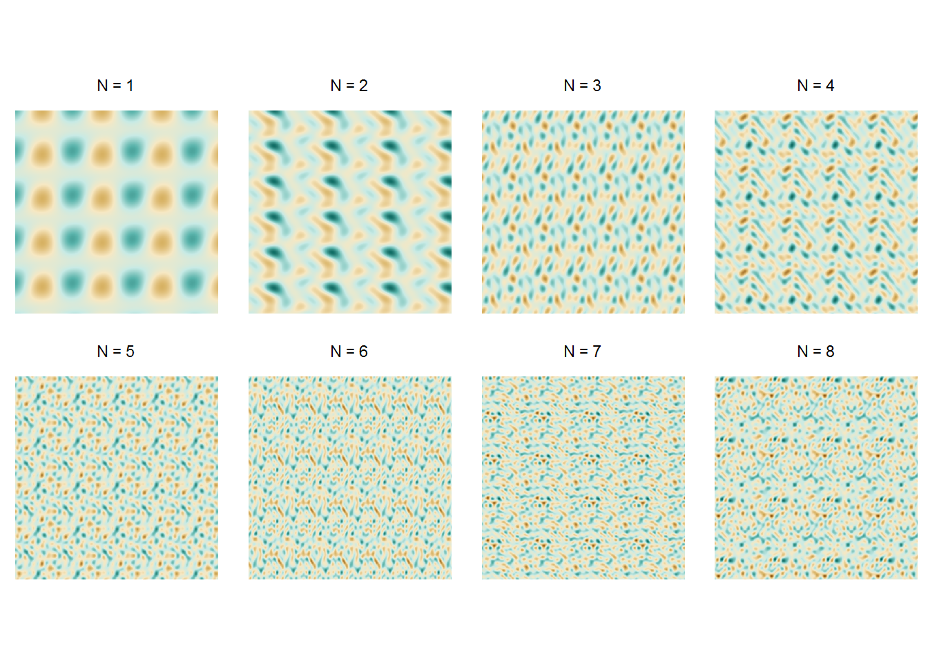

Walking through a 3D space painted with a Fourier series

Finally, we are going to take advantage of the periodic nature of Fourier series to build a nice GIF that will smoothly loop without glitches. We do this by evaluating the function in a 3D grid, and then slicing the space along a path defined by one of the 3 coordinates. Specifically, for this animation we will sample a truncated Fourier series with known periods, and then we will navigate along the $z$ axis for a full period.

# function parameters 
N = 1 # number of harmonics
P_z = 2*pi # period for the z dimension
l = P_z/2 # limits for (x, y) dimensions

# animation parameters
steps = 100 # how many frames
res = 480 # size of image = res x res

f_s_3d = get_fourier_series(N = N, d = 3, P = rep(P_z, 3))

# build data
df_grid_3d =
  expand.grid(
    x = seq(-l, l, length.out = res),
    y = seq(-l, l, length.out = res),
    t = 1:steps,
    KEEP.OUT.ATTRS = FALSE
  ) %>%
  as_data_frame() %>%
  # add z variable for each step
  inner_join(
    data.frame(t = 1:steps,
               z = seq(0, P_z, length.out = steps))
    , by = "t") %>%
  # multidplyr::partition(t) %>% 
  mutate(s = f_s_3d(cbind(x, y, z))) %>% 
  select(-z) # %>% 
  # collect()

The above process is slow and tedious, but it can be trivially parallelized by using the package multidplyr with the addition of a couple of extra lines of codes. However, I couldn’t get blogdown to work with a cluster, but you can try it at home by un-commenting the last lines in the chunk.

Below is the resulting animation. Isn’t its smoothness relaxing?

# plot
p = df_grid_3d %>%
  ggplot(aes(x = x, y = y, frame = t)) +
  geom_raster(aes(fill = s), show.legend = FALSE) +
  scale_fill_gradient(low = "black", high = "white") +
  coord_fixed() +
  theme_void()

# animate
gganimate(plot        = p,
          title_frame = FALSE)

Final remarks

In this post I have given a brief introduction to real-valued Fourier series in higher dimensions. I gave a practical demonstration of the concept by visualizing functions for the cases where $d\in \{2, 3\}$ . I think that this seemingly “useless” concept of making pretty pictures of mathematical objects can be very enlightening, because it gives you a more intuitive grasp of the underlying concepts.