BIDC: Bayesian Inference for Default Correlations
I just released a package on Github called BIDC, which stands for Bayesian Inference for Default Correlations. I started working on this together with my colleague Victor Medina back when I was a financial stability analyst at the Superintendency of Banks and Financial Institutions in Chile. In fact, you can see the slides from our presentation at the 2017 version of SBIF conference here (Biron and Medina 2017). The difference is that, instead of Stan, the method available in BIDC uses a Metropolis-Hastings-within-Gibbs MCMC sampler (Gilks 1996) written entirely in base R, that runs much faster. Currently, it only supports the naive version shown on those slides.
Description
BIDC is a package that aims to provide multiple tools for performing Bayesian inference on the default correlation of a given portfolio, along with any other latent factor. Currently, we support only one model, but we would like to expand this in the future.
The available model is a generalization of the finite version of the Vasicek model for correlated defaults in a credit portfolio (Vasicek 1987, Vasicek (2002)), which allows for clients with different probabilities of default (PD). Also, we assume a uniform prior on $\rho$:
\[ \begin{aligned} \rho &\sim \text{U}(0,1) \\ M_t &\overset{iid}{\sim} \mathcal{N}(0,1) \\ y_{it}|\rho, M_t, P_{it} &\overset{ind}{\sim} \text{Bernoulli}\left( \Phi\left( \frac{\Phi^{-1}(P_{it}) - M_t\sqrt{\rho}}{\sqrt{1-\rho}} \right)\right) \end{aligned} \]
The main data input corresponds to a matrix $Y$ of size $N\times T$, where $T$ is the amount of periods observed and $N$ is the number of individuals observed each period, which for simplicity we assume constant. Then, $Y$ contains a value of 1 at position $(n,t)$ if at time $t$ the n-th client defaulted.
As explained in (Biron and Medina 2017), in order to infer $(\rho, \{M_t\}_t)$ we use the assumption that the PDs are exogenous. Hence, the user needs to supply anothe matrix $P$ of the same dimensions as $Y$, which at the position $(n, t)$ should containt a good estimate of the PD for the corresponding value in $Y$. Assuming exogenous PDs has the benefit that we can leverage PD models which are commonplace both in financial institutions and regulatory agencies. However, the price to pay, as is the case with all models fitted in two stages, is that the uncertainty will be underestimated. The alternative would be to fit the PDs (or rather $\Phi^{-1}(P_{it})$) jointly with $(\rho, \{M_t\}_t)$, as shown in McNeil and Wendin (2007). We prefer to focus on modelling the dependence structure of the defaults.
It is crucial to understand that $Y$ is exchangeable within columns: for $t_1 \neq t_2$, the value at $(n, t_1)$ is not necessarily associated with the same client that the value at $(n, t_2)$ is. In other words, we could reshufle each column and still obtain the same information. However, the matrix $P$ has to be reshuffled in the same way to maintain consistency.
To sample from the posterior distribution, we use a Metropolis-Hastings-within-Gibbs approach. We need to use MH steps because the full conditionals are not analytically tractable. However, all the updates are one-dimensional, so that the algorithm does not face the difficulties that
Example
Let us start by defining a function that will let us obtain simulated data. We simulate the latent factors $\{M_t\}_t$ as coming from an AR(1) process, so that the output resembles a business cycle.
Note that the function returns the binary matrix $Y$, and also the actual PDs used to sample $Y$.
sample_data = function(N, Tau, rho, median_pd, a){
  # N: number of individuals
  # Tau: time steps
  # rho: default correlation
  # median_pd: median marginal probability of default
  # a: AR(1) param for M_t process
  # output: list with: y  : matrix size N \times Tau of integers in (0,1)
  #                    p_d: matrix size N \times Tau of PDs

  # sample M_t process
  M = numeric(Tau)
  M[1L] = rnorm(1L)
  for(tau in 2L:Tau) M[tau] = a*M[tau-1L] + sqrt(1-a^2)*rnorm(1L)

  # sample critical values
  x_c = matrix(rnorm(N*Tau, mean = qnorm(median_pd)),
               nrow = N)

  # sample y_it
  y = matrix(NA_integer_, nrow = N, ncol = Tau)
  for(tau in 1L:Tau) {
    prob = pnorm((x_c[,tau]-sqrt(rho)*M[tau])/sqrt(1-rho))
    y[,tau] = 1L*(runif(N) <= prob)
  }

  p_d = pnorm(x_c) # probit to get probabilities
  return(list(y=y,p_d=p_d))
}
Now we sample the actual data. We set a value of $\rho=0.15$.
set.seed(1313)

# parameters for simulated data
N = 1000L # number of individuals
Tau = 100L # time steps
rho = 0.15 # default correlation
median_pd = 0.25 # median marginal probability of default
a = 0.9 # AR(1) param for M_t process

# get data
l_data = sample_data(N=N,Tau=Tau,rho=rho,median_pd=median_pd,a=a)
We are now ready to run the chain. We will do this for 1,000 iterations. Note that we will supply the exact PDs that were used to simulate the data. This is the best case scenario for our method.
library(BIDC)

S = 1000L # number of iterations
start_time = proc.time()
chain = bidc_pd(S=S, y=l_data$y, p_d=l_data$p_d, verbose = 0L)
print(proc.time() - start_time)
##    user  system elapsed
##  93.254   0.068  93.338
Trace plots
The trace plot for $\rho$ show that the chain converges rapidly to a region close to the true value, and then slows down.
suppressPackageStartupMessages(library(dplyr))
suppressPackageStartupMessages(library(tidyr))
suppressPackageStartupMessages(library(ggplot2))

chain[,c(1L, Tau, Tau+1L)] %>%
  as.data.frame() %>%
  setNames(c("M_1", paste0("M_", Tau), "rho")) %>%
  mutate(s = seq_len(nrow(.))) %>%
  gather(select = -"s") %>%
  ggplot(aes(x = s, y = value, colour = key)) +
  geom_line(show.legend = FALSE) +
  facet_wrap(~key, scales = "free_y", ncol = 1L) +
  labs(x = "Iteration",
       y = "Value")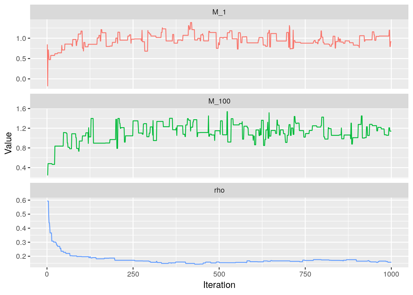
Confidence band for $M_t$
chain[,-(Tau+1L)] %>%
  as_tibble() %>%
  setNames(1L:ncol(.)) %>%
  mutate(s=1L:nrow(.)) %>%
  gather("tau", "M", select = -s) %>%
  mutate(tau=as.integer(tau)) %>%
  group_by(tau) %>%
  summarise(qtiles = list(data.frame(
    q   = c(".025", ".975"),
    val = quantile(M, c(0.025, 0.975)),
    stringsAsFactors = FALSE
  ))) %>%
  ungroup() %>%
  unnest() %>%
  spread(q, val) %>%
  ggplot(aes(x=tau, ymin=`.025`, ymax=`.975`, fill = "1")) +
  geom_ribbon(show.legend = FALSE) +
  labs(x = "Time",
       y = "95% posterior band for M_t")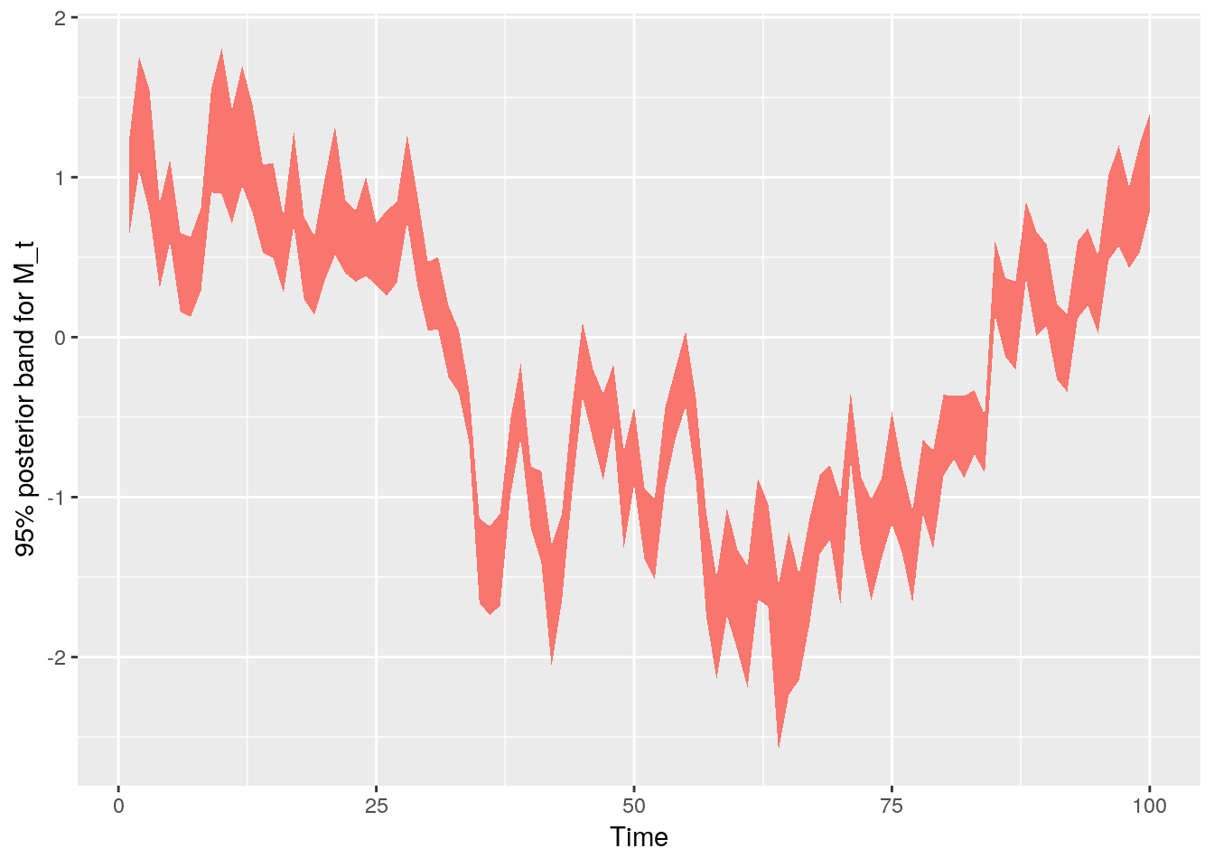
Example with bad estimates of the PD
Now, we are going to run the chain again, but instead of using the true PDs, we will feed it a noisy version which is shrunken towards the median PD with a random mixing coefficients $c_{it}$: \[
\tilde{P}_{it} = c_{it}\text{PD}_{\text{median}} + (1-c_{it})P_{it}
\]
This is to demonstrate that the current approach is very sensitive to the quality of the PDs used. We draw the $c_{it}$ from a Beta distribution that is centered around 0.2. We do this type of perturbation because we assume that, even though the user might have a bad PD model, it will at least be able to estimate well the overall PD.
b = 100; m = 0.2
a = (m*(b-2) + 1)/(1-m) # forces the mode of the beta to be at m
mix_c = matrix(rbeta(N*Tau, shape1 = a, shape2 = b), nrow = N)
p_d_noisy = mix_c*median_pd + (1-mix_c)*l_data$p_d
chain = bidc_pd(S=S, y=l_data$y, p_d=p_d_noisy, verbose = 0L)
Trace plots
We see now that the trace for $\rho$ is very far away from the true value.
chain[,c(1L, Tau, Tau+1L)] %>%
  as.data.frame() %>%
  setNames(c("M_1", paste0("M_", Tau), "rho")) %>%
  mutate(s = seq_len(nrow(.))) %>%
  gather(select = -"s") %>%
  ggplot(aes(x = s, y = value, colour = key)) +
  geom_line(show.legend = FALSE) +
  facet_wrap(~key, scales = "free_y", ncol = 1L) +
  labs(x = "Iteration",
       y = "Value")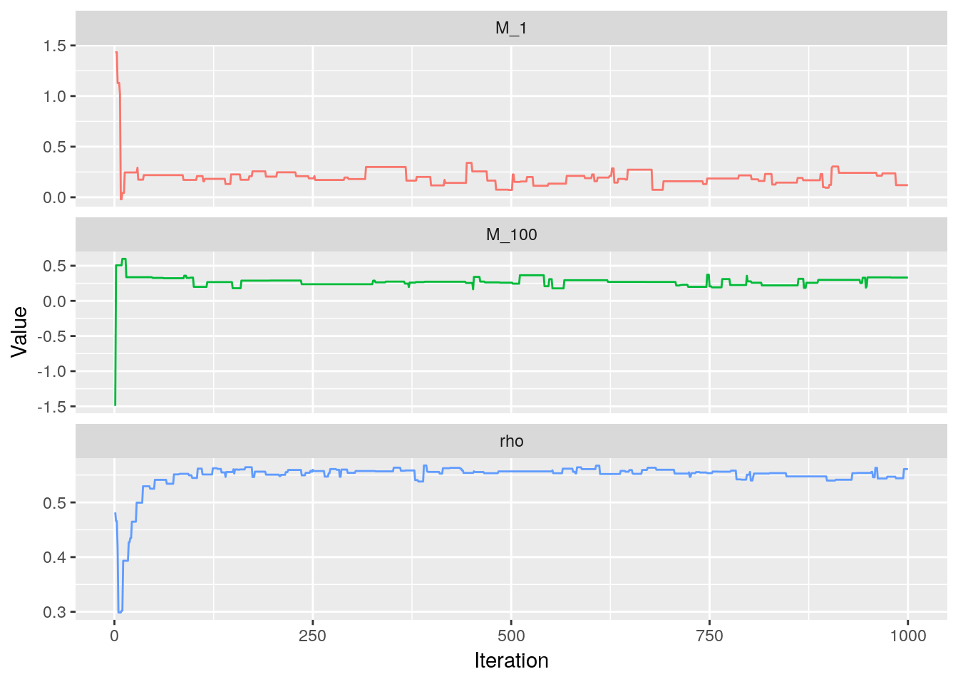
Confidence band for $M_t$
Compare this with the case of perfect information from above: the shape is very similar, but the values are shrunken towards 0.
chain[,-(Tau+1L)] %>%
  as_tibble() %>%
  setNames(1L:ncol(.)) %>%
  mutate(s=1L:nrow(.)) %>%
  gather("tau", "M", select = -s) %>%
  mutate(tau=as.integer(tau)) %>%
  group_by(tau) %>%
  summarise(qtiles = list(data.frame(
    q   = c(".025", ".975"),
    val = quantile(M, c(0.025, 0.975)),
    stringsAsFactors = FALSE
  ))) %>%
  ungroup() %>%
  unnest() %>%
  spread(q, val) %>%
  ggplot(aes(x=tau, ymin=`.025`, ymax=`.975`, fill = "1")) +
  geom_ribbon(show.legend = FALSE) +
  labs(x = "Time",
       y = "95% posterior band for M_t")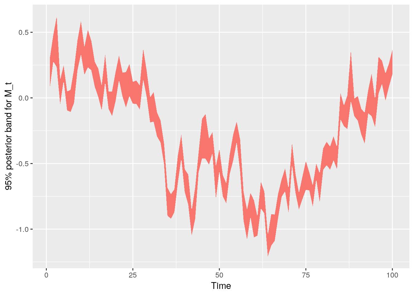
Conclusions
I hope I have been able to show how the method in this package can be used to quickly obtain estimates for the default correlation of a portfolio. Hopefully, this “hello world” method that is made available in this release will serve as a motivation for me and others to propose more interesting models and algorithms.
References
Biron, Miguel, and Victor Medina. 2017. “Leveraging Probability of Default Models for Bayesian Inference of Default Correlations.” Paper presented at 3rd Conference on Banking Development, Stability, and Sustainability, Santiago, Chile. https://www.sbif.cl/sbifweb/servlet/ConozcaSBIF?indice=C.D.A&idContenido=16698.
Gilks, Walter R. 1996. Markov Chain Monte Carlo in Practice. Chapman & Hall: London.
McNeil, Alexander J, and Jonathan P Wendin. 2007. “Bayesian Inference for Generalized Linear Mixed Models of Portfolio Credit Risk.” Journal of Empirical Finance 14 (2). Elsevier: 131–49.
Vasicek, Oldrich Alfons. 1987. “Probability of Loss on Loan Portfolio.” KMV Corporation Technical Report.
———. 2002. “The Distribution of Loan Portfolio Value.” Risk 15 (12): 160–62.