New member in SBGLM: sparse linear regression

Description of the model

This is a very basic Bayesian linear regression model, with a minor twist that lets us impose sparsity in the effects: $$ \begin{aligned} \sigma_b^2 &\sim \text{Inv-Gamma}(s_b, r_b) \\ \sigma_e^2 &\sim \text{Inv-Gamma}(s_e, r_e) \\ \pi &\sim \text{Beta}(s_1, s_2) \\ \beta_k|\sigma_b^2 &\overset{iid}{\sim} \mathcal{N}(0, \sigma_b^2) \\ z_k|\pi &\overset{iid}{\sim} \text{Bernoulli}(\pi) \\ y|\beta, z, X, \sigma_e^2 &\sim \mathcal{N}(X(\beta \odot z), \sigma_e^2 I_N) \end{aligned} $$

where $\odot$ is the Hadamard (element-wise) product of two vectors, $y$ is the vector of responses of length $N$, and $X$ is a matrix of covariates of size $N\times P$. As you can see, the way sparsity is introduced is by “masking” or “switching on and off” components of $\beta$ using the binary variables $z$. Thus, the effect of a given covariate $x_k$ on the response will be $\beta_k z_k$, and not just $\beta_k$.

The oldest reference I know about this way of introducing sparsity in a Bayesian model is Griffiths and Ghahramani (2011), although the technique might be older. I actually discovered it by myself, so I was glad when I saw that people had already been using it. Also, I’m almost sure that this is just an equivalent way of implementing the spike-and-slab prior, so that is why probably nobody mentions it as something new.

The posterior distribution is obtained by using a Gibbs sampler, which is easy to derive given the conjugacies present in the model. Everything is implemented using only base R, which I try to promote in order to minimize dependency issues in the future.

As with all things Bayesian, the beauty of this model resides in its assessment of uncertainty, since asymptotically (in MCMC runs) exact post-selection inference comes for free, something that for frequentist methods like Lasso (Tibshirani 1996) or the Elastic Net (Zou and Hastie 2005) has only very recently been made possible (see for example Lee et al. (2016)). Recall that the brute-force alternative for evaluation of post-selection uncertainty in such models was to bootstrap your dataset, having to do a full cross-validation search of parameters for each run. Needless to say, this quickly becomes unfeasible.

Indeed, the posterior distribution $p(\beta \odot z|\mathcal{D})$ of the effects, where $\mathcal{D} = \{y, X\}$, contains all the relevant information for assessing uncertainty by explicitly accounting for the introduction of sparsity. In fact, the posterior $p(z|\mathcal{D})$ of the switches themselves is also interesting, as it reveals the joint probability that each of the covariates is included in the model.

Gibbs updates

In order to construct the Gibbs sampler, the first thing to notice is that, conditional on $z$, the model actually reduces to a standard Bayesian linear regression, where the design matrix is now $X_{:A}$, with $A=\{k: z_k=1\}$ being the active set of covariates. Thus, the Gibbs updates in the sparse model for the active coefficients and the variances are exactly the same as for the standard model.

Recall that the update for $\beta$ in a standard linear regression requires a matrix inversion. Here, we also face that problem. However, because we only do this for the active components, then as long as $|A|$ is small (~100) this implementation runs in surprisingly reasonable times, regardless of how large $P$ can be. In the future, I would like to test if having element-wise updates could be used to tackle larger problems, at the expense of perhaps having slower mixing times.

The inactive components $\beta_{-A}$ still have to updated, though. It is easy to show that the full conditional is equal to the prior. This is very intuitive, because they are being disconnected from the model by their switches, so there is no information from the data that can be used to update our belief about them.

The update for the switches is the only one that is trickier to derive, so I leave it here for future reference: $$ \frac{\mathbb{P}(z_k=1|-, \mathcal{D})}{\mathbb{P}(z_k=0|-, \mathcal{D})} = \exp \left( \log \pi -\log(1-\pi) - \frac{\beta_k}{2\sigma_e^2} \left[ -2(X^Ty)_{k} + \beta_k (X^TX)_{kk} + 2(X^TX)_{:k}^T(\beta \odot z_0) \right] \right) $$

where $z_0$ is equal to $z$ but has a 0 at the $k$-th position. Note that the computations that are expensive ($X^Ty, X^TX$) have to be calculated once and stored so that they’re available for re-use.

Finally, the update for $\pi$ follows from the standard Beta-Bernoulli conjugacy: $$ \pi|z \sim \text{Beta}\left(s_1 + \sum_k z_k, s_2 + P - \sum_k z_k \right) $$

Example: simulated data

My intention here is to show you how this model performs by applying it to a simulated dataset. The data generating process is actually a modified version of one of the simulations that Zou and Hastie (2005) used to evaluate the Elastic Net. Their approach had a minor mistake, which I pointed out in my report about this paper. However, the fundamental ideas are the same: to assess the behavior of the model under the situation $N \ll P$, where only a few of the available covariates are relevant, and also when those variables are clumped into groups with high within-group correlation and between-group independence. This is achieved by creating groups of covariates from slightly perturbed sine functions, with each group having a different frequency. This way, we ensure that the covariates are uncorrelated. The problem with the method in the Elastic Net paper was that it wrongly used groups of constant features, so that the within-group correlation was actually 0, not as intended. Finally, all the variables in the relevant groups are assigned the same coefficient, and the rest are assigned a beta equal to 0.

Hopefully, the following code is clear enough so that the ideas of the previous paragraph are evident:

get_data = function(N, P, nz_P, n_groups, b_val, sigma_b, sigma_e){
  # define beta
  p = nz_P %/% n_groups
  beta = numeric(P)
  beta[seq_len(nz_P)] = b_val
  
  # define groups of highly correlated variables
  # the lowest sigma_b is, the highest the within-group correlation
  X = do.call(cbind,
              lapply(seq_len(n_groups),
                     function(u) {
                       matrix(rep(sin(u * (1:N)), p), ncol=p) +
                         matrix(rnorm(N*p, sd= sigma_b), nrow=N)
                     }))
  
  # append many noise covariates
  X = cbind(X, matrix(rnorm(N*(P-nz_P)), nrow = N))
  
  # get response
  y = as.vector(X %*% beta) + rnorm(N, sd = sigma_e)
  
  return(list(X=X, y=y))
}

Now we sample the data. The following plot shows the correlation matrix for the first 150 of the total 500 covariates, which shows exactly the pattern that we would expect.

set.seed(1313)

N = 200L # number of observations
P = 500L # total number of covariates
nz_P = 45L # number of covariates with nonzero coefficients
n_groups = 5L # number of groups of covariates (nz_P/n_groups within each)
b_val = 3 # value of the effect for nonzero coefficients
sigma_b = 0.1 # noise added to covariates in the same group
sigma_e = 5 # noise in the response

dta = get_data(N, P, nz_P, n_groups, b_val, sigma_b, sigma_e)

# visualize correlations
M = cor(dta$X[,seq_len(150L)])
M = t(apply(M, 2, rev))
op = par(mar = rep(0, 4))
image(M, axes=FALSE, asp = 1, useRaster = TRUE)

par(op)

Now we are ready to run the Gibbs sampler on this data:

library(SBGLM)

S=2000L
results = sblm_gibbs(
  X       = dta$X,
  y       = dta$y,
  S       = S,
  verbose = 200L
)

## Chain initialized. Beginning iterations!
## 
## Iteration 200: |A| = 11, sigma_2_e = 28.42, sigma_2_b = 122.48
## Iteration 400: |A| = 14, sigma_2_e = 25.95, sigma_2_b = 65.07
## Iteration 600: |A| = 12, sigma_2_e = 28.80, sigma_2_b = 67.35
## Iteration 800: |A| = 10, sigma_2_e = 30.75, sigma_2_b = 250.25
## Iteration 1000: |A| = 10, sigma_2_e = 32.57, sigma_2_b = 182.99
## Iteration 1200: |A| = 12, sigma_2_e = 29.33, sigma_2_b = 203.41
## Iteration 1400: |A| = 9, sigma_2_e = 27.43, sigma_2_b = 215.18
## Iteration 1600: |A| = 11, sigma_2_e = 30.91, sigma_2_b = 81.36
## Iteration 1800: |A| = 12, sigma_2_e = 28.91, sigma_2_b = 220.84
## Iteration 2000: |A| = 11, sigma_2_e = 35.74, sigma_2_b = 194.41

Great! Let us plot the traces for $\pi$ and the variances to check that everything is running as it should:

suppressPackageStartupMessages(library(dplyr))
library(tidyr)
library(ggplot2)

t(sapply(results, function(l){
  c(l$pi_z, l$sigma_2_e, l$sigma_2_b)
})) %>%
  as.data.frame.matrix() %>%
  setNames(c("Pi", "sigma_2_e", "sigma_2_b")) %>%
  mutate(Iteration = seq_len(S)) %>%
  gather("key", "Value", select = -Iteration) %>%
  ggplot(aes(x = Iteration, y = Value, color = "1")) +
  geom_line(show.legend = FALSE) +
  scale_y_log10() +
  theme_bw() +
  facet_wrap(~key, scales = "free_y", ncol = 1L)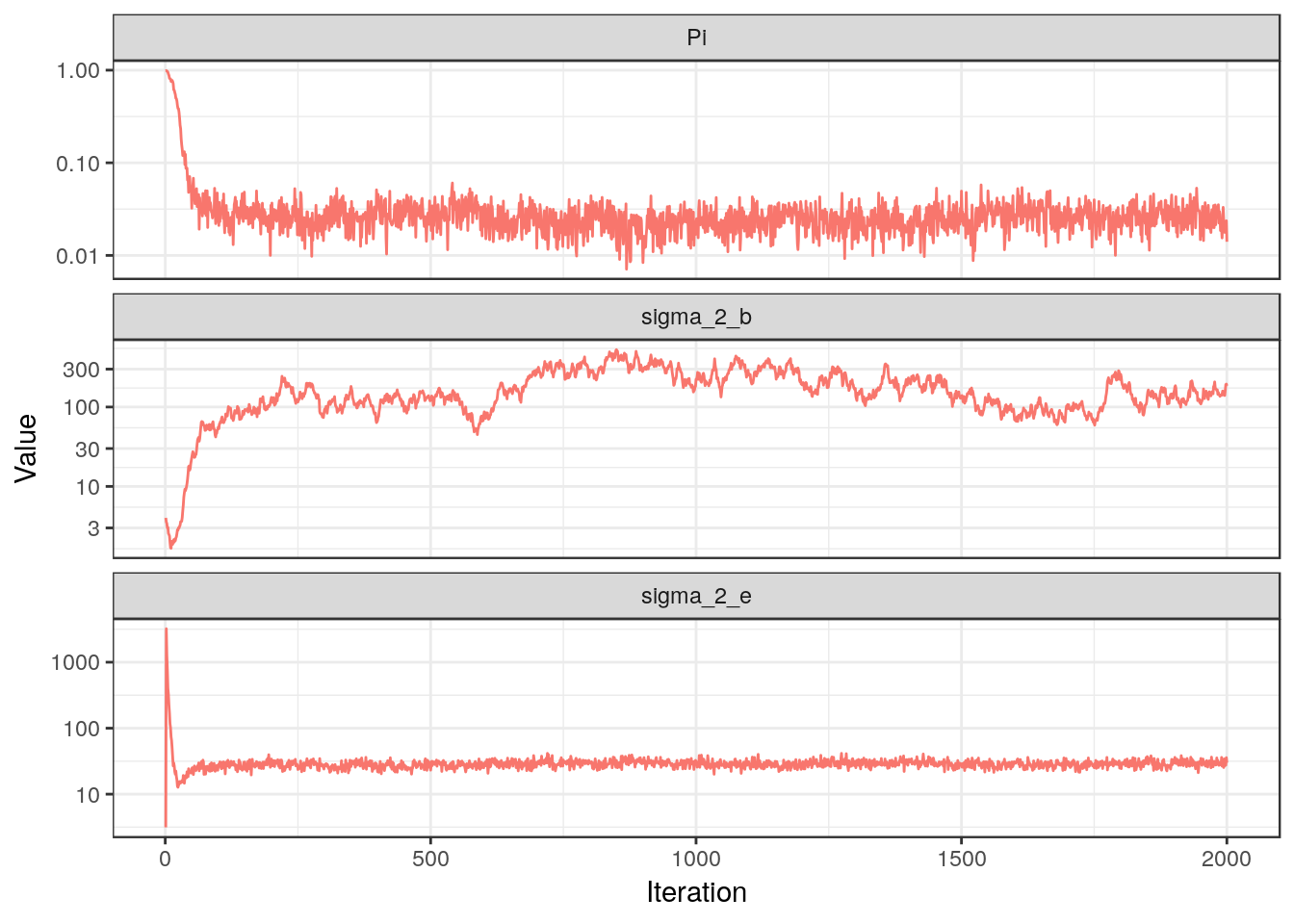

For $\pi$ and $\sigma_e^2$ we see the nice “fuzzy caterpillar” pattern that should emerge, and in fact both of them settle very quickly close to their true values. For $\sigma_b^2$, however, we observe a more random-walk behavior. Since its update depends only on the active coefficients, we now plot some of them:

t(sapply(results, function(l){l$beta[c(5L, 40L, 140L)]})) %>%
  as.data.frame.matrix() %>%
  setNames(paste("Beta", c(5L, 40L, 140L))) %>%
  mutate(Iteration = seq_len(S)) %>%
  gather("key", "Value", select = -Iteration) %>%
  ggplot(aes(x = Iteration, y = Value, color = "1")) +
  geom_line(show.legend = FALSE) +
  theme_bw() +
  facet_wrap(~key, scales = "free_y")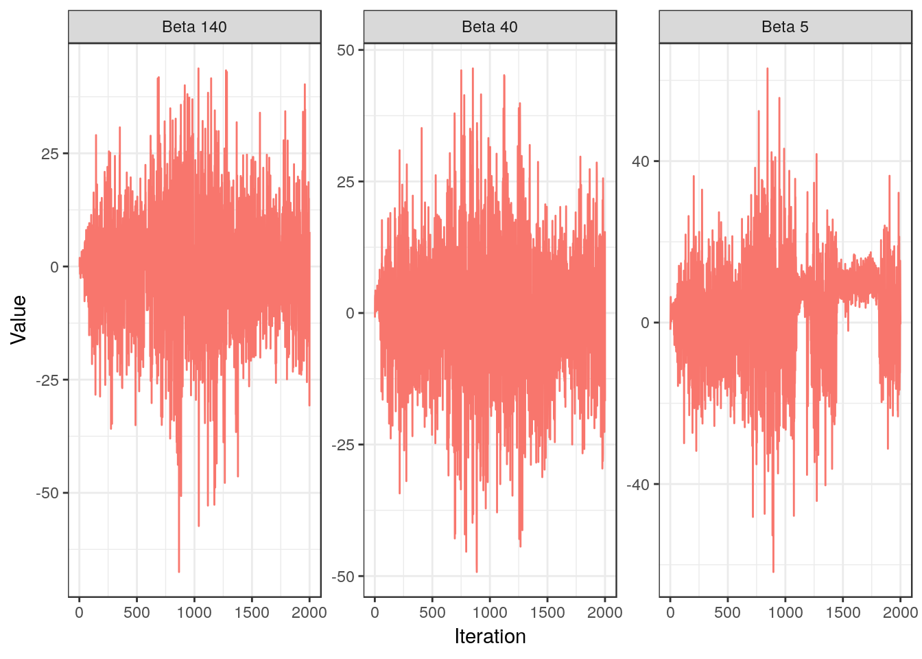

For $\beta_{40}$ and $\beta_{140}$ there doesn’t seem to be any problem. We wouldn’t expect issues for the latter anyway, since it is not relevant for the model and therefore is updated using the prior. We do note that $\beta_{5}$, which is in the true model, exhibits again a random-walk behavior.

In order to dig deeper into this issue, we will construct a plot that focuses on the first group of variables $(\beta_1,...,\beta_9)$, by assessing the contribution that each of them make to their sum. The sum is a relevant quantity because the covariates they represent are almost exact copies, so it is meaningful to talk about a “total” effect arising from the group.

# colorblind palette
# http://www.cookbook-r.com/Graphs/Colors_(ggplot2)/#a-colorblind-friendly-palette
cbbPalette <- c("#000000", "#E69F00", "#56B4E9", "#009E73", "#F0E442", "#0072B2", "#D55E00", "#CC79A7")

sel_beta = seq_len(nz_P %/% n_groups)
trace_beta = sapply(results, function(l){l$beta[sel_beta]})
trace_z = sapply(results, function(l){sel_beta %in% l$A})
t(trace_beta * trace_z) %>%
  as.data.frame.matrix() %>%
  setNames(sel_beta) %>%
  mutate(Iteration = seq_len(S)) %>%
  gather("key", "Value", select = -Iteration) %>%
  ggplot(aes(x = Iteration, y = Value, fill = key)) +
  geom_area(show.legend = FALSE) +
  geom_hline(yintercept = b_val * (nz_P %/% n_groups), linetype = "dashed") +
  scale_fill_manual(name = "", values = c(cbbPalette, "navyblue")) +
  theme_bw()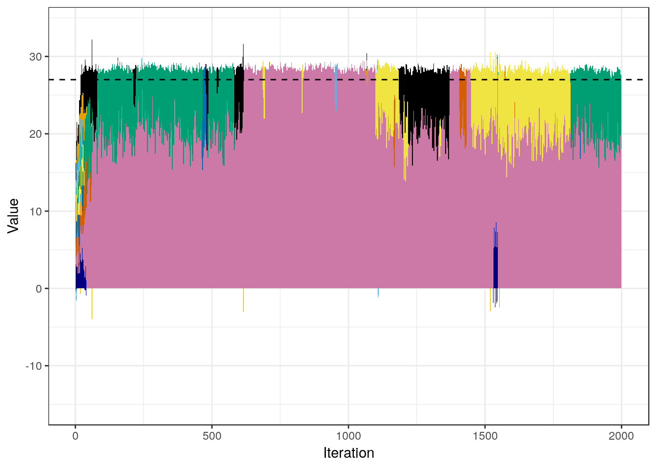

Note how the sum total of the 9 components quickly approaches the expected value of 9 $\times$ 3 $=$ 27 (highlighted with the dashed line in the plot), and then stays very close to it. However, there is a sort of non-stationary dynamic in which the model never actually settles on any particular combination of the components. This is, of course, expected, given the extremely high correlation that the covariates within the group have. In other words, the sampler has a very good idea about where the total contribution of the group is, but it has a hard time inferring how to allocate this effect among the components, given the little data there is. In turn, because one coefficient gets assigned the effect of many others, the magnitudes of the components of $\beta$ varies considerably, and this “confusion” propagates back to $\sigma_b^2$ which explains its behavior.

The above phenomenon should not be unexpected, given the high within-group correlation and the fact that $N \ll P$. Even though the predictions of the model won’t be affected (the fact that $\sigma_e^2$ is correctly recovered is evidence of this), one should always be cautious when interpreting the contributions of each variable to the response variable, given that the effects of highly correlated variables cannot be disentangled easily, especially with few data.

To finish this analysis, let us plot the posterior probability of each covariate being included in the model. The vertical line shows the limit for the active set:

sapply(results[seq.int(S%/%2L+1L, S, 1L)], function(l){
  z=logical(P)
  z[l$A]=TRUE
  z
}) %>%
  rowMeans() %>%
  as.data.frame() %>%
  setNames(c("prob")) %>%
  mutate(Variable = seq_len(P)) %>%
  ggplot(aes(x = Variable, y = prob)) +
  geom_line(show.legend = FALSE) +
  geom_vline(xintercept = nz_P, linetype = "dotted") +
  theme_bw() +
  labs(y = "Posterior probability of inclusion")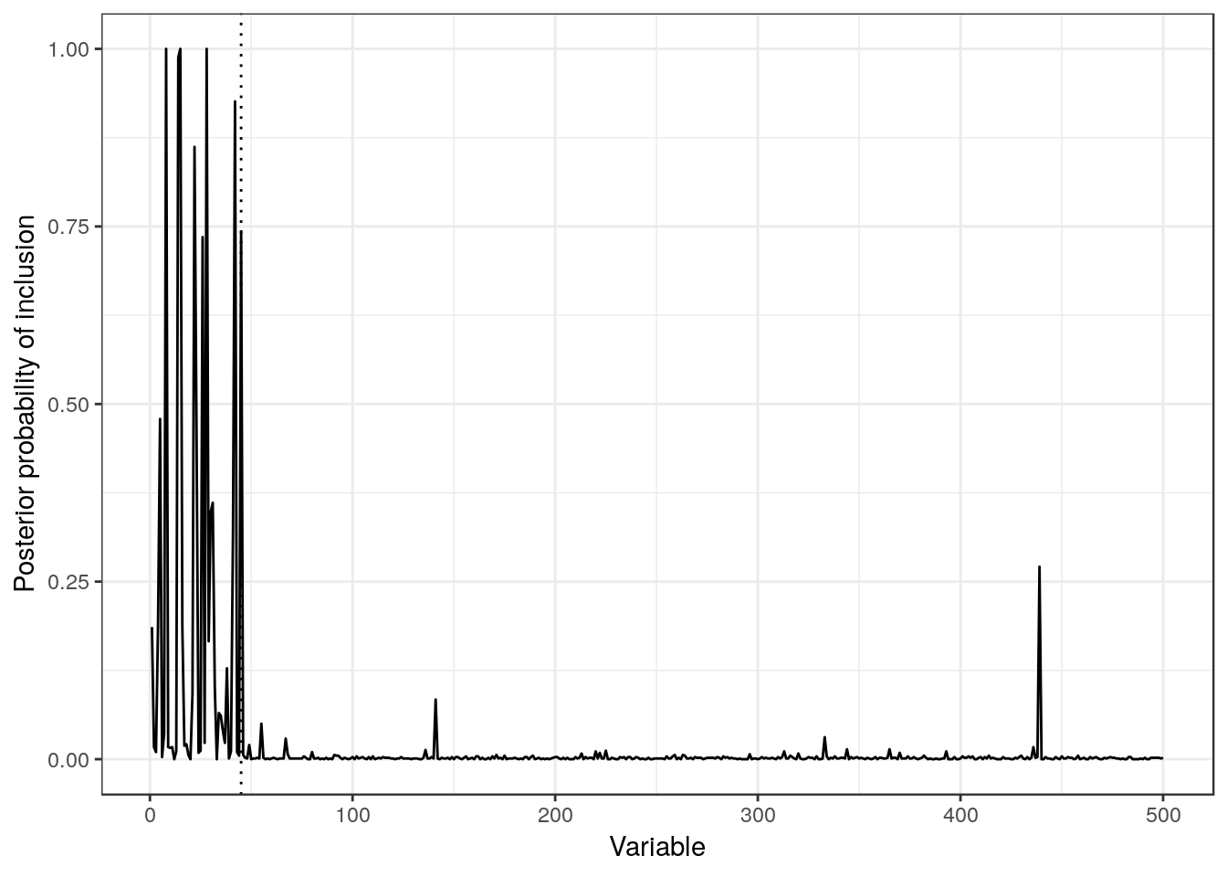

Given the symmetries present in the data, we would expect a uniform probability of inclusion of the first 45 variables (active set), and then close to 0 probability for the rest. The latter assumption holds almost perfectly, except for one variable at the end with a quite high probability of inclusion. On the other hand, we see a non-uniform probability of inclusion among the true relevant covariates, which is consistent with the problems previously described.

Conclusions

In this post I wanted to be a party-pooper, by fitting the sparse Bayesian linear regression to a terrible dataset, showing how it manages to work in some aspects, but fails to deliver in the most difficult ones. Even though this was obviously expected, it is important to stress how disconnected from the “reality” can the coefficients inferred from this type of data be. As always, it is good to know the limitations of our methods.

Feel free to leave a comment below!

References

Griffiths, Thomas L, and Zoubin Ghahramani. 2011. “The Indian Buffet Process: An Introduction and Review.” Journal of Machine Learning Research 12 (Apr): 1185–1224.
Lee, Jason D, Dennis L Sun, Yuekai Sun, Jonathan E Taylor, and others. 2016. “Exact Post-Selection Inference, with Application to the Lasso.” The Annals of Statistics 44 (3). Institute of Mathematical Statistics: 907–27.
Tibshirani, Robert. 1996. “Regression Shrinkage and Selection via the Lasso.” Journal of the Royal Statistical Society. Series B (Methodological). JSTOR, 267–88.
Zou, Hui, and Trevor Hastie. 2005. “Regularization and Variable Selection via the Elastic Net.” Journal of the Royal Statistical Society: Series B (Statistical Methodology) 67 (2). Wiley Online Library: 301–20.